Relative Entropy Pathwise Policy Optimization - Technical Overview

tl;dr: Try our REPPO algorithm, it’s great and incredibly stable! Our code is available at https://github.com/cvoelcker/reppo

This blog post serves as a lightweight, and hopefully somewhat entertaining, introduction to our new algorithm, Relative Entropy Pathwise Policy Optimization. If you want the full formal overview with proper references, fewer anecdotes, and more rigorous notation, please check out our paper as well.

For readers interested in “how“ we built REPPO (the technical bits), please refer to the first section. If you are simply curious “where” you can use REPPO, we offer the second section with some advice for practitioners (this will be updated in the future from feedback). Finally, we offer some additional details and ideas for follow-up research in our addendum on Discrete REPPO. If you want to read a more tongue-in-cheek discussion of my personal motivations for designing REPPO, check out our blogpost on “why” we built REPPO.

How we designed REPPO

If we want to design a good on-policy algorithm, the first thing we have to do is take the current champion, PPO, seriously! PPO is fast, easy to implement, and can be tuned in almost any environment. So we want to keep these strengths. This is one place where many RL researchers have failed. I myself have designed better algorithms that are incredibly sample efficient (check out MAD-TD ;) ), but complex and slow to train. We don’t want to do that here. We want an algorithm that matches PPO in speed and simplicity, but improves on it in terms of reliability and performance. So with these goals, let us explore REPPO!

The REPPO backbone

The core algorithmic skeleton of REPPO will look very, very familiar to everybody who is comfortable with PPO. Remember, we are keeping it simple and will keep building on strength ;). We have an environment interaction phase, compute value targets with a GAE-style estimator (except that we compute values and not advantages), and then interleave several epochs of value and policy updates on the gathered batch of data. We actually coded REPPO by taking a PPO codebase and replacing components until we got REPPO.

We will now walk through these changes, explain how to build them, and why they improve over PPO. Algorithmic We will first go over the algorithmic components of REPPO, the loss functions and why we introduce them. If you already know all about PPOs problems with gradient variance, you can skip the first part.

Why is PPO brittle?

There are two core concepts that PPO uses: a REINFORCE style policy gradient and clipped importance sampling. Both together are the key culprits behind both its success and its brittleness.

There are already so many good explanations behind REINFORCE (or score-based gradient estimators, as we call them in our paper), so I won’t repeat too much here. I’ve always been partial to this very thorough overview by Lilian Weng https://lilianweng.github.io/posts/2018-04-08-policy-gradient/, so go read it in case you are interested. Pay attention to the part about the deterministic policy gradient, it’s going to come up in a bit. And do come back once you are finished ;) !

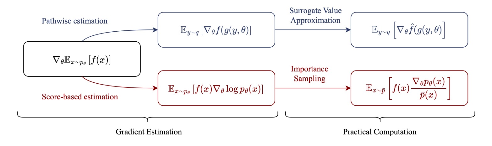
Basically, the REINFORCE trick allows us to compute gradients of expectations where the distribution itself depends on the parameters:

\[\nabla_\theta J(\theta) = \nabla_\theta \int p_\theta(x) J(x)\, dx = \int p_\theta(x) J(x)\, \nabla_\theta \log p_\theta(x)\, dx.\]

However, this estimator comes with two distinct problems: first, it is known to have rather high variance, which strongly affects the behavior of the resulting RL algorithms. Many different methods have been developed to decrease this variance, mostly relying on baselines, or control variates if you want to be fancy. However, the second issue quickly comes into play: resampling. In principle, once we have collected our data, estimated our gradient, and taken a single gradient step, we have to recollect a fresh new batch of data, as our policy has changed. That is absurdly expensive and slow, even with fast simulators. Instead, we can adjust for the fact that we are estimating an expectation with old samples from a past policy by importance sampling:

\[\mathbb{E}_{p(x)}[f(x)] = \mathbb{E}_{q(x)}\!\left[\frac{p(x)}{q(x)} f(x)\right].\]

This allows us to do multiple updates with the same samples, at the cost of introducing even more variance. As the old behavioral (or data-gathering) policy slowly shifts away from the current policy, the importance ratio \(\pi/\pi_\mathrm{old}\) can grow very quickly when not carefully controlled¹. PPOs core contribution is, in fact, a mechanism to prevent this ratio from growing out of control, clipping the update when the ratio becomes too large. However, this comes at the cost of slow updates.

What if we could get rid of both the high variance gradient estimator and importance sampling in one fell swoop?

We will replace the REINFORCE style policy gradient with reparameterization! Skip the next part if you are familiar with reparameterization! (We are skipping a lot of stuff today for the experts, but I like being thorough for the newcomers).

Introducing reparameterization

Instead of relying on the policy gradient theorem to derive a policy gradient, we can take an alternate route: reparameterization. A policy is reparameterizeable (a horrible word that may not actually be in the dictionary?) when you can “move out” the sampling from the computational graph. That sounds complicated, and is best explained by a short example: imagine our policy as a Gaussian with parameters \(\mu_\theta\) and \(\sigma_\theta\) that both depend on our state $x$. Our action needs to be sampled as \(a \sim \mathcal{N}(\mu(x), \sigma(x))\), which is not a differentiable operation. However, I can also write my action as \(a = \mu(x) + \sigma(x) * \epsilon\) where \(\epsilon\) is random noise sampled from a standard normal distribution. I can write this as \(a = g(\mu_\theta, \sigma_\theta, \epsilon)\) and computing \(\nabla_\theta g\) is a simple autodiff operation. We have essentially made the randomness an input to our function. This allows us to rewrite our policy gradient as

\[\nabla_\theta J(\theta) \\ = \nabla_\theta \mathbb{E}_{a \sim \pi_\theta}[J(x,a)] \\ = \nabla_\theta \mathbb{E}_{\epsilon \sim \mathcal{N}}[Q(x,g(\mu_\theta,\sigma_\theta,\epsilon))] \\ = \mathbb{E}_{\epsilon \sim \mathcal{N}}[\nabla_\theta Q(x,g(\mu_\theta,\sigma_\theta,\epsilon))].\]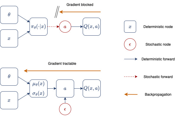

However, to use reparameterization, we need one more step. Our objective, J is the return from the environment under our policy, and (normally) not directly differentiable. This is where we use a second trick: substituting a surrogate return estimator. In more common parlance, this is a learned state-action value function, or Q function. Experienced readers will see that we have now gathered (almost) all the elements that make up the SAC algorithm, and in many ways, REPPO can simply be thought of as On-policy SAC++².

Now, having a learned Q function almost magically allows us to get around the second cause of high variance as well: we can get rid of importance sampling. Importance sampling was needed, originally, because we cannot get return estimates for our updated policy. But with the trained value function we can, we simply need to query the value function at a new action \(a’ \sim \pi_{\theta’}\)! Now we can do multiple update steps without having to deal with exploding importance ratios!

We visualized a tiny toy example of the behavior of different gradient approximations below:

So we just take SAC and run on-policy with it? Not quite! The on-policy nature of our algorithm will quickly come and haunt us.

Policy and Critic Training

Q value learning normally relies on a replay buffer of past experience, but on-policy learning generates a lot of data. And to be fast, we need to keep our data on the GPU. So unless we want to use a couple of H100s, we need an alternative plan.

The first step is to update our Q functions on-policy. This actually makes our training setup easier than SAC or comparable algorithms, as many of the instability issues in SAC arise from off-policy training. We can forgo target networks, clipped double-Q learning and other shenanigans, since on-policy targets are quite stable. To do this in practice, we repurpose the GAE computation in PPO and compute a Generalized Q Estimate. A very similar setup was recently proposed for Parallel Q Networks, a similar algorithm to ours, which we will discuss again at the end. Our policy can now be updated by maximising the Q function with regard to the policy:

\[\theta_{\text{new}} = \theta - \eta \nabla_\theta \mathbb{E}_{a \sim \pi_\theta}[-Q(x,a)].\]

Dealing with limited memory, and too little and too much policy change

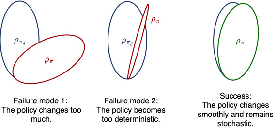However, we now need to deal with two problems: constraining the distribution shift, and keeping policy entropy high. Our Q function is only accurate on states and actions that we have actually seen recently. So while we can resample and forgo importance sampling in our policy objective, we still have to constrain the policy to not move too far away from the behavior policy. We do this by enforcing a relative entropy constraint, or trust-region. Basically, we prevent the updated policy from moving further than a fixed KL distance from the behavior policy. This is not a new idea, many, many other algorithms attempt to do this. However, we make it easy!

Instead of complicated Hessian approximations, as in TRPO, clipping, as in PPO, or ignoring the issue, as in SAC, we approximate the KL from samples and add it as a second objective to our policy update. This requires us to set a hyperparameter \(\lambda_\mathrm{KL}\) which we will get to in a second. For now let us write down our policy objective as

\[\theta_{\text{new}} = \theta - \eta \nabla_\theta \\ \mathbb{E}_{a \sim \pi_\theta}\!\Big[-Q(x,a)\Big] \\ + \lambda_{\text{KL}} \, KL_{\text{approx}}[\pi_\theta \,\|\, \pi_{\theta_{\text{old}}}].\]

However, simply constraining the KL divergence to the data-gathering policy creates a problem. Over the course of the optimization, we can get stuck with too little entropy in our policy. As the strength of the KL term is dependent on the entropy, we can reach a point where the behavior policy has a very small entropy. Then any change in policy causes very large KL values, which prevents further policy updates.

This leads us to our second major component: maximum entropy reinforcement learning. Again, we are not going to dive into the details here, as many great papers and surveys have been written about the topic, but we will briefly summarize the core idea. In addition to penalizing the KL deviation between our current policy and the behavior policy, we also prevent our policy from becoming too deterministic. This update nicely ensures that we have some noise in our policy which will be used for exploration. Our policy objective now becomes

\[\theta_{\text{new}} = \theta - \eta \nabla_\theta \\ \mathbb{E}_{a \sim \pi_\theta}\!\Big[-Q(x,a)\Big] \\ + \lambda_{\text{KL}} \, KL_{\text{approx}}[\pi_\theta \,\|\, \pi_{\theta_{\text{old}}}] \\ - \lambda_{\mathcal{H}} \, \mathcal{H}(\pi_\theta).\]

Maximum entropy RL also requires that we include the entropy term in the Q function. This means our Q learning loss is

\[\mathcal{L}(Q_\phi; x,a,r,x') = \Big(Q(x,a) - \big[r + \gamma Q(x',a') - \log \pi(a'|x')\big]\Big)^2.\]

This should be very familiar if you are comfortable with SAC and similar algorithms.

Balancing the loss terms

We have one major problem remaining: the hyperparameters \(\lambda_\mathrm{KL}\) and \(\lambda_\mathcal{H}\). These govern how important the policy constraints are compared to the actual policy objective, maximising the Q function. In PPO, the entropy parameter is normally set to a fixed value, while the policy objective is clipped once the KL deviation becomes too large. In SAC on the other hand, the entropy multiplier is automatically tuned. To do this, the second SAC paper introduces another hyperparameter, the target entropy (I promise, this will simplify things soon :D). Now we measure if the current policy is equal to the target entropy. If not, we increase the value of \(\lambda_\mathcal{H}\), making it more important to increase the entropy. If the entropy is too large, we reduce the value of \(\lambda_\mathcal{H}\). The nice thing about this scheme is that setting a target value for the entropy turns out to be easier than setting an appropriate multiplier. As we train our RL policy, the magnitude of the Q values change, and so if we fix the parameter \(\lambda_\mathcal{H}\) we might end up with too much entropy in the beginning when Q is small, and too little in the end when Q is large. A target entropy is invariant to the magnitude of the Q function, which means less tuning.

Now the perceptive among you might ask: can we do the exact same thing with \(\lambda_\mathrm{KL}\). And the answer is yes, we absolutely can! The really cool thing is that tuning both parameters keeps everything nice and balanced: neither entropy nor KL collapses, so the agent always keeps exploring.

The fascinating thing about the REPPO KL scheme is that the original PPO paper actually evaluates a very similar KL constraint and autotuning scheme as we use here. But they don’t use an entropy target! This means that while the KL constraint is well controlled, the overall amount of change in the policy is not, as it changes with the entropy. Tuning both together is a crucial step in making everything work!

Architectural changes to Q function learning

In addition to the algorithmic changes, there are a couple of neural network architectural tricks which we introduce to make our Q functions as precise as possible. Remember, as we rely on surrogate Q values for our policy updates, we need these Q values to be as precise as possible. While we use three tricks in the published REPPO version, I am only going to present one of them in detail, as it contributes the most to precise Q value training: categorical Q losses.

Stopping regression: Categorical Q learning

Categorical losses for Q learning have been a trick for a while, but I don’t fully know where they originate. I read about them for the first time in the MuZero paper. Since then, they have been used in Dreamer-v3, TD-MPC2, and finally formally evaluated and described by Jesse Farebrother in “Stop regressing”. Since I couldn’t find a nice blog post to link, I’ll actually explain some details here!

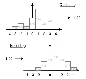The core idea is to represent the Q value as a histogram \(h(x,a)\) so that \(\mathbb{E}[h(x,a)] = Q(x,a)\). To achieve this, we first compute a regular Q target as \(T_Q = r +\gamma Q\). Then, we embed this scalar as a histogram. Normally, a uniform or log scale is used for the value of each bin, and the distribution is chosen heuristically. MuZero and Dreamer v3 use two-hot encodings: the bins to the left and right of the true target get all the weight so that the expectation is the true target. In HL-Gauss, which we use, the histogram approximates a Gaussian with \(\mu = T_Q\) and fixed standard deviation. The visualization on the left shows the encoding and the decoding process. Note that curiously, decoding and re-encoding do not lead to the same distribution.

The Q function histogram is updated using a cross entropy loss. We interpret the histogram as a target distribution and minimize the KL between our prediction and the embedded target value. Why should this work better than a regular squared loss? We actually don’t fully know, although there is a lot of speculation! So consider this an interesting opportunity for research ;)

But even though we don’t fully know why this trick works so well, we can empirically observe that it does!

Other implementation details: normalization and auxiliary tasks

Normalization has been all the rage in off-policy RL, and for good reasons. It can help to prevent catastrophic overestimation, and with some formal finagling, it can be shown to prevent the issues of the deadly triad* (*Side note: While the PQN paper makes a big deal about stabilizing off-policy learning, PQN does not keep old data around for a very long time. We achieve almost identical returns with on-policy learning, and don’t require normalization, so the benefits of off-policy learning might disappear if you don’t actually keep old data in your replay buffer). However, as we are on-policy, not all of these issues apply to REPPO. We still find some benefits from using simple layer norms in our networks. We also normalize the input data, which has a much larger effect and (speculative) could be related to the recent success of BatchNorm and the CrossQ algorithm.

Further, we chose to implement auxiliary tasks, similar to those used in the recent off-policy setup MrQ. Again, we find that these help somewhat, but are not crucial for performance.

How you can use REPPO

One of our core design goals for REPPO was that it is almost a drop-in replacement for PPO. As stated, the algorithmic backbone (the way in which data is gathered and the policy and values are updated) is very similar, so practitioners should have little trouble replacing one with the other without changing too much about the general setup. Just check out the github repository 😉 .

However, we can give you some tuning advice: in general, we want large batches and relatively long rollouts for the data collection phase. This stabilizes Q learning, which is slightly more important in REPPO compared to PPO. In addition, you might need slightly larger neural networks for your value, for the same reason.

The really fascinating thing about REPPO so far is that we haven’t really needed to retune any hyperparameters other than the environment dependent ones (such as reducing the discount factor \(\gamma\) in environments with shorter horizons). The only thing that has had a strong impact are the GAE discount factor \(\lambda_\mathrm{GAE}\), which we needed to reduce in the Atari Learning Environments to \(0.65\) from our default value of \(0.95\). In discrete environments, our returns have more variance, so a smaller GAE parameter will reduce the impact of this variance on the critic update.

Other than that we found that for harder tasks, such as the humanoid control tasks in the new mujoco playground benchmark, larger data batches can lead to better performance. In general, it makes sense to use the largest batch sizes you can reasonably afford before you observe slowdowns.

On torch vs jax

We provide REPPO implementations in both torch and jax. However, the jax version is a lot faster than the torch version, most likely due to the way the static graph is compiled. We found that the torch version is unable to fully take advantage of frameworks such as torch.compile. Our leading hypothesis is that, since we require a lot of random sampling, we run into an issue with torch. Random sampling forces a GPU-CPU sync in torch, which slows down the algorithm(Since none of us are CUDA experts, we are not a hundred percent sure that this is the only, or even the main problem facing torch REPPO. If you are a CUDA expert and want to do a deep dive on this, shoot us a mail.). We are currently working on providing code to connect frameworks which are built for fast torch experimentation, such as maniskill and IsaacLab, efficiently to our jax algorithm.

Conclusion

Use REPPO! Hopefully this blog post has been entertaining and informative, and motivated you to try your hand at our new algorithm. And like I said, the best part is that we can still provide hands-on help. Just shoot us a mail or open a github issue.

Addendum: Discrete REPPO (D-REPPO)

Normally, reparameterization cannot be trivially applied to categorical or discrete variables. The full reason for this is technical, but any existing estimator leads to a biased gradient. This is an annoying limitation since one of the strengths of PPO is its broad applicability, and we want to keep this! However, luckily we can circumvent this problem!

Notice that we are trying to differentiate

\[\mathbb{E}_{a \sim \pi_{\theta}(\cdot|x)}[Q(x,a)]\]

with samples from \(\pi\). However, in the discrete case, we do not have to sample at all, we can compute the expectation in closed from

\[\mathbb{E}_{a \sim \pi_{\theta}(\cdot|x)}[Q(x,a)] = \sum_{a \in A} \pi(a|x) Q(x,a).\]

This is a differentiable expression, and so we can simply substitute it into our loss. We still “count” this as fundamentally following REPPO, because, in essence, differentiating the expectation directly is simply the limit of getting infinitely many samples from our policy distribution. So, strictly speaking, this is even better!

We benchmarked our D-REPPO variant against PQN and found that while it performs pretty much on par, we are losing out somewhat in terms of exploration. It seems that entropy based exploration is not quite enough to get SOTA performance in Atari games. This opens up exciting avenues for future research: can we use some tricks, for example the V-Trace algorithm, to get better exploration policies that cover more interesting parts of the state space? We leave this question to you, dear interested reader, and look forward to your follow up work!